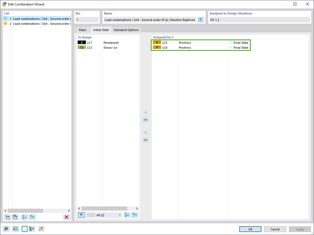
The combination wizard provides you with the option to consider more than one initial state. RFEM and RSTAB allow you to specify different initial states (prestress, form-finding, strain, and so on) for the target combinations in the combinatorics.
You can thus, for example, generate load states on the basis of a form-finding analysis with varying imperfections.
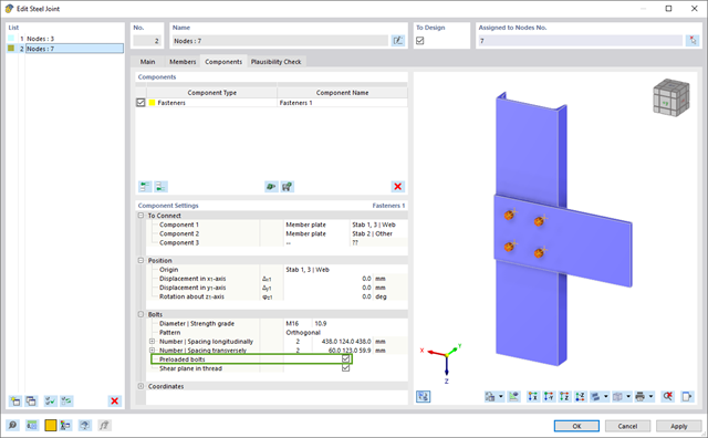
In the Steel Joints add-on, you have this option to consider the preloaded bolts in the calculation of all components.
You can easily activate the prestress using the check box in the bolt parameters, and it has an impact on the stress-strain analysis as well as the stiffness analysis.
Go to Explanatory Video
The Ponding load type allows you to simulate rain actions on multi-curved surfaces, taking into account the displacements according to the large deformation analysis.
This numerical rainfall process examines the assigned surface geometry and determines which rainfall portions drain away and which rainfall portions accumulate in puddles (water pockets) on the surface. The puddle size then results in a corresponding vertical load for the structural analysis.
For example, you can use this feature in the analysis of approximately horizontal membrane roof geometries subjected to rain loading.
Go to Explanatory Video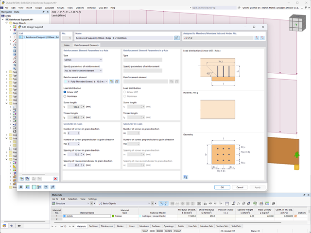
Did you know? In the Design Supports, you can now define fully threaded screws as transversal compression stiffening elements for the "Compression Perpendicular to Grain" design. In this case, the pressing-in and buckling of the bolts is analyzed.
Moreover, the design shear resistance is checked in the plane of the screw tip. The angle of dispersal can be considered as linear under 45° or nonlinear (according to Bejtka, I. (2005). Verstärkung von Bauteilen aus holz mit vollgewindeschrauben. KIT Scientific Publishing.).
.png?mw=640&hash=55038d2a1591f62179796666cb9b2fede0274e19)
A graphical and tabular output of the results for deformations, stresses, and strains helps you when determining the soil solids. To achieve this, use the special filter criteria for targeted selection of results.
The program doesn't leave you alone with the results. If you want to graphically evaluate the results in the soil solids, you can use the guide objects. For example, you can define clipping planes. This allows you to view the corresponding results in any plane of the soil solid.
And not just that. The utilization of result sections and clipping boxes facilitates the precise graphical analysis of the soil solid.
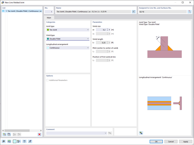
In RFEM 6, it is possible to define line welds between surfaces and to calculate the weld stresses using the Stress-Strain Analysis add-on.
The following joint types are available:
- Butt Joint
- Corner joint
- Lap Joint
- T-joint
Depending on the selected joint type, you can select the following weld types:
- Single Square
- Double Square
- Double Bevel
- Single V
- Double V
- Single U
- Double U
- Single J
- Double J

Enter and model a soil solid directly in RFEM. You can combine the soil material models with all common RFEM add-ons.
This allows you to easily analyze the entire models with a complete representation of the soil-structure interaction.
All parameters required for the calculation are automatically determined from the material data that you have entered. The program then generates the stress-strain curves for each FE element.

Do you want to model and analyze the behavior of a soil solid? To ensure this, special suitable material models have been implemented in RFEM.
You can use the modified Mohr-Coulomb model with a linear-elastic ideal-plastic model or a nonlinear elastic model with an oedometric stress-strain relation. The limit criterion, which describes the transition from the elastic area to that of the plastic flow, is defined according to Mohr-Coulomb.

The stress and strain results by surface can be output in the surface result table according to the thickness layer.
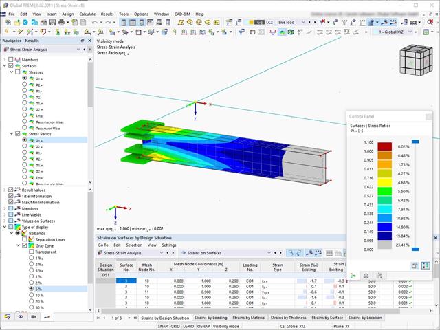
For stress-strain analyses, it is possible to define gray zones for nonrelevant value ranges in the result panel.
- Design of tension, compression, bending, shear, torsion, and combined internal forces
- Consideration of a notch
- Design of compression perpendicular to the grain on the end and intermediate supports with (EC 5) and without reinforcement elements (fully threaded screws)
- Optional shear force reduction at the support (see the Product Feature)
- Design of curved and tapered members
- Consideration of higher strengths for similar components that are close together (factor ksys according to EN 1995‑1‑1, 6.6(1)-(3))
- Option to increase shear resistance for softwood timber according to DIN EN 1995‑1‑1:NA NDP to 6.1.7(2)
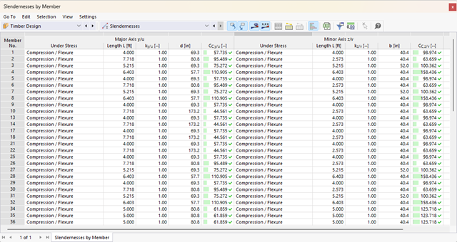
- Stability analyses for flexural buckling, torsional buckling, and flexural-torsional buckling under compression
- Import of the effective lengths from the calculation using the Structure Stability add-on
- Graphical input and check of the defined nodal supports and effective lengths for stability analysis
- Determination of the equivalent member lengths for tapered members
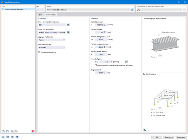
- Consideration of Lateral-Torsional Bracing Position
- Lateral-torsional buckling analysis of the structural components subjected to moment loading
- Depending on the standard, a choice between user-defined input of Mcr, analytical method from the standard, and use of internal eigenvalue solver
- Consideration of a shear panel and a rotational restraint when using the eigenvalue solver
- Graphical display of a mode shape if the eigenvalue solver was used
- Stability analysis of structural components with the combined compression and bending stress, depending on the design standard
- Comprehensible calculation of all necessary coefficients, such as the factors for considering moment distribution or interaction factors
- Alternative consideration of all effects for the stability analysis when determining internal forces in RFEM/RSTAB (second-order analysis, imperfections, stiffness reduction, possibly in combination with the Torsional Warping (7 DOF) add-on)
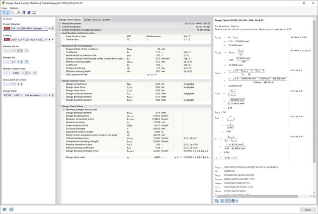
- Arbitrary definition of the charring time
- Option to calculate with or without adhesion of the layer for surface structures (cross-laminated timber)
- Free user-defined specification of the fire parameters
- Consideration of Different Effective Lengths in Fire Resistance Design
- Optional design "Compression perpendicular to grain"
- Graphical result display integrated in RFEM/RSTAB, such as a design ratio
- Complete integration of the results into the RFEM/RSTAB printout report
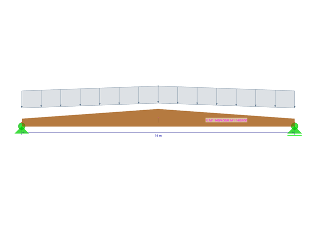
Your options in timber design are diverse. You can consider cut-to-grain angles, transverse tension stresses, and volume-dependent radii of curvature for tapered and curved members. To design the area of the grain cut, the strength is adjusted accordingly in the case of bending tension or bending pressure. In order to also allow you to perform a stability analysis with the equivalent member method, the height to determine the effective and lateral-torsional buckling lengths is set at a distance of 0.65 × h to the actual design point.
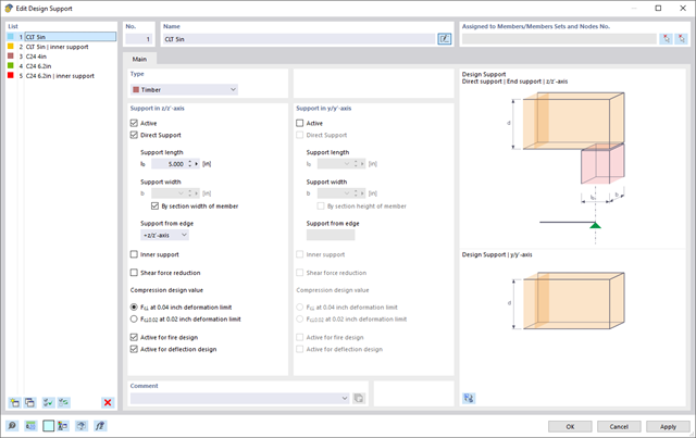
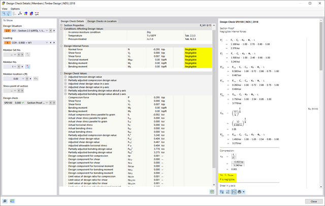
Here you have a free choice. You can perform the support pressure design at any point for the loading in the y- and z-directions of a cross-section. You are free to differentiate between inner and outer supports. A factor kc,90 for the pressure perpendicular to the grain can be user-defined (for example, 1.75 for glued-laminated timber). If allowed, the support length is increased automatically according to the standard specifications. This allows you to achieve a more efficient design with minimum effort.

Did you know? In contrast to other material models, the stress-strain diagram for this material model is not antimetric to the origin. You can use this material model to simulate the behavior of steel fiber-reinforced concrete, for example. Find detailed information about modeling steel fiber-reinforced concrete in the technical article about Determining the material properties of steel-fiber-reinforced concrete.
In this material model, the isotropic stiffness is reduced with a scalar damage parameter. This damage parameter is determined from the stress curve defined in the Diagram. The direction of the principal stresses is not taken into account. Rather, the damage occurs in the direction of the equivalent strain, which also covers the third direction perpendicular to the plane. The tension and compression area of the stress tensor is treated separately. In this case, different damage parameters apply.
The "Reference element size" controls how the strain in the crack area is scaled to the length of the element. With the default value zero, no scaling is performed. Thus, the material behavior of the steel fiber concrete is modeled realistically.
Find more information about the theoretical background of the "Isotropic Damage" material model in the technical article describing the Nonlinear Material Model Damage.
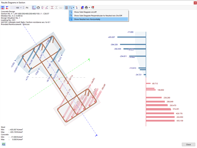
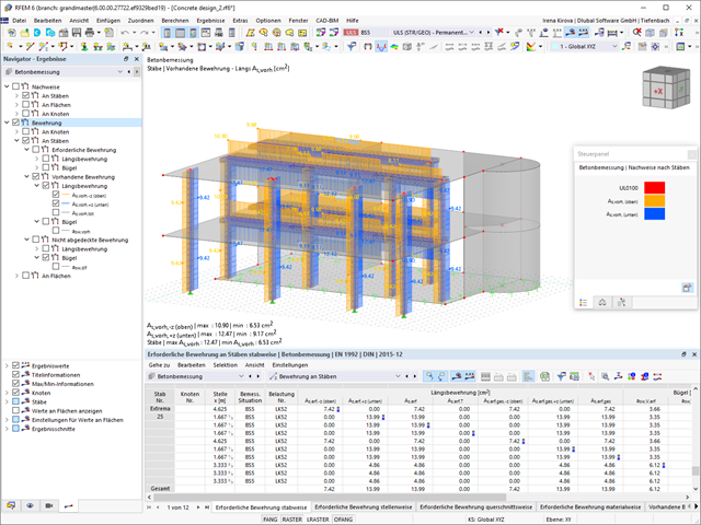
You can display the existing stresses and strains of a concrete cross-section and the reinforcement as a 3D stress image or 2D graphic. Depending on which results do you select in the result tree of the design details, the stresses or strains are displayed to you in the defined longitudinal reinforcement under the load actions or the limit internal forces.

- Calculation of stationary incompressible turbulent wind flow using the SimpleFOAM solver from the OpenFOAM® software package
- Numerical scheme according to the first and second order
- Turbulence models RAS k-ω and RAS k-ε
- Consideration of surface roughness depending on model zones
- Model design via VTP, STL, OBJ, and IFC files
- Operation via bidirectional interface of RFEM or RSTAB for importing model geometries with standard-based wind loads and exporting wind load cases with probe-based printout report tables
- Intuitive model changes via drag & drop and graphical adjustment assistance
- Generation of a shrink-wrap mesh envelope around the model geometry
- Consideration of environmental objects (buildings, terrain, and so on)
- Height-dependent description of the wind load (wind speed and turbulence intensity)
- Automatic meshing depending on a selected depth of detail
- Consideration of layer meshes near the model surfaces
- Parallelized calculation with optimal utilization of all processor cores of a computer
- Graphical output of the surface results on the model surfaces (surface pressure, Cp coefficients)
- Graphical output of the flow field and vector results (pressure field, velocity field, turbulence – k-ω field, and turbulence – k-ε field, velocity vectors) on Clipper/Slicer planes
- Display of 3D wind flow via animated streamline graphics
- Definition of point and line probes
- Multilingual user interface (German, English, Czech, Spanish, French, Italian, Polish, Portuguese, Russian, and Chinese)
- Calculations of several models in one batch process
- Generator for creating rotated models to simulate different wind directions
- Optional interruption and continuation of the calculation
- Individual color panel per result graphic
- Display of diagrams with separate output of results on both sides of a surface
- Output of the dimensionless wall distance y+ in the mesh inspector details for the simplified model mesh
- Determination of the shear stress on the model surface from the flow around the model
- Calculation with an alternative convergence criterion (you can select between the residual types pressure or flow resistance in the simulation parameters)
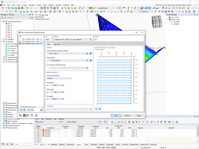
To model structures in RWIND Basic, you find a special application in RFEM and RSTAB. Here, you define the wind directions to be analyzed by means of related angular positions about the vertical model axis. At the same time, you define the elevation-dependent wind profile on the basis of a wind standard. In addition to these specifications, you can use the stored calculation parameters to determine your own load cases for a stationary calculation per each angular position.
As an alternative, you can also use the RWIND Basic program manually, without the interface application in RFEM or RSTAB. In this case, RWIND Basic models the structures and terrain environment directly from the imported VTP, STL, OBJ, and IFC files. You can define the height-dependent wind load and other fluid-mechanical data directly in RWIND Basic.
Discover the new features in RFEM and RSTAB for the determination of wind loads using RWIND:
- Useful load wizards for generating wind load cases with different flow fields in different wind directions
- Wind load cases with freely assignable analysis settings including a user-defined specification of the wind tunnel size and wind profile
- Comprehensive display of the wind tunnel with input wind profile and turbulence intensity profile
- Visualization and use of the RWIND simulation results
- Global definition of a terrain (horizontal planes, inclined plane, table)

Our webinars are recorded, and you can refer to them at any time. View the webinars about RFEM and RSTAB as well as the add-ons.
Webinars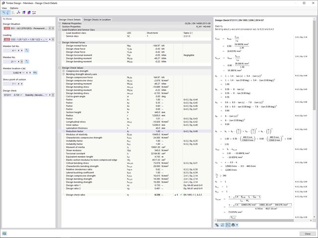
Compared to the RF‑/TIMBER Pro add-on module (RFEM 5 / RSTAB 8), the following new features have been added to the Timber Design add-on for RFEM 6 / RSTAB 9:
- In addition to Eurocode 5, other international standards are integrated (SIA 265, ANSI/AWC NDS, CSA O86, GB 50005)
- Design of compression perpendicular to grain (support pressure)
- Implementation of eigenvalue solver for determining the critical moment for lateral-torsional buckling (EC 5 only)
- Definition of different effective lengths for design at normal temperature and fire resistance design
- Evaluation of stresses via unit stresses (FEA)
- Optimized stability analyses for tapered members
- Unification of the materials for all national annexes (only one "EN" standard is now available in the material library for a better overview)
- Display of cross-section weakenings directly in the rendering
- Output of the used design check formulas (including a reference to the used equation from the standard)
Compared to the RF‑/ALUMINUM add-on module (RFEM 5 / RSTAB 8), the following new features have been added to the Aluminum Design add-on for RFEM 6 / RSTAB 9:
- In addition to Eurocode 9, the US standard ADM 2020 is integrated.
- Consideration of the stabilizing effect of purlins and sheets by rotational restraints and shear panels
- Graphical display of the results in the gross section
- Output of the used design check formulas (including a reference to the used equation from the standard)

Compared to the RF‑SOILIN add-on module (RFEM‑5), the following new features have been added to the Geotechnical Analysis add-on for RFEM 6:
- Creation of the layered soil as a 3D model from the entirety of the defined soil samples
- Recognized material law according to Mohr-Coulomb for soil simulation
- Graphical and tabular output of stresses and strains at any depth of the soil
- Optimal consideration of the soil-structure interaction on the basis of an overall model

Compared to the RF‑/STEEL add-on module (RFEM 5 / RSTAB 8), the following new features have been added to the Stress-Strain Analysis add-on for RFEM 6 / RSTAB 9:
- Treatment of members, surfaces, solids, welds (line welded joints between two and three surfaces with subsequent stress design)
- Output of stresses, stress ratios, stress ranges, and strains
- Limit stress depending on the assigned material or a user-defined input
- Individual specification of the results to be calculated through freely assignable setting types
- Non-modal result details with prepared formula display and additional result display on the cross-section level of members
- Output of the design check formulas used

The form-finding process gives you a structural model with active forces in the "prestress load case" This load case shows the displacement from the initial input position to the form-found geometry in the deformation results. In the force or stress-based results (member and surface internal forces, solid stresses, gas pressures, and so on), it clarifies the state for maintaining the found form. For the analysis of the shape geometry, the program offers you a two-dimensional contour line plot with the output of the absolute height and an inclination plot for the visualization of the slope situation.
Now, a further calculation and structural analysis of the entire model is performed. For this purpose, the program transfers the form-found geometry including the element-wise strains into a universally applicable initial state. You can now use it in the load cases and load combinations.
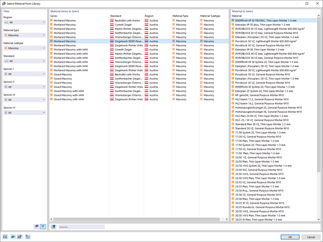
You enter and model the structure directly in RFEM. You can combine the masonry material model with all common RFEM add-ons. This enables you to design the entire building models in connection with masonry.
The program automatically determines for you all parameters required for the calculation by using the material data that you have entered. Then, it finally generates the stress-strain curves for each FE element.
The program can also help you here. It determines the bolt forces on the basis of the calculation on the FE model and evaluates them automatically. You can perform the design checks of the bolt resistance for the failure cases tension, shear, hole bearing, and punching shear according to the standard. The program takes care of everything else in this step. It determines all the necessary coefficients and displays them clearly.
- Do you want to perform weld design? The required stresses are also determined on the FE model in that case. Then, the Weld element is modeled as elastic-plastic shell element, where every FE element is checked for its internal forces. (Plasticity criteria is set to reflect failure acc. to AISC J2-4 and J2-5 (weld resistance check) and also J2-2 (base metal capacity check). The design can also be carried out with the partial safety factors according to the selected National Annex.
You can perform the plate design plasticall by comparing the existing plastic strain to the allowable plastic strain. By default this is set to 5% for the AISC 360 but can be specified through user-definition 5% according to EN 1993-1-5, Annex C, or again, user-defined specification.
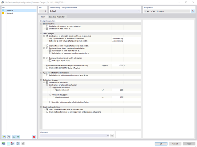
Are you looking for a deformation calculation? Check the Serviceability Configuration, where it can be activated. You can also control the consideration of long-term effects (creep and shrinkage) and tension stiffening between cracks in the dialog box above. The creep coefficient and shrinkage strain are calculated using the specified input parameters, or you can define them individually.
Furthermore, you can specify the deformation limit value individually for each structural component. The max. deformation is defined as the allowable limit value. In addition, you have to specify whether you want to use the undeformed or the deformed system for the design check.
The standards already specify the approximation methods (for example, deformation calculation according to EN 1992‑1‑1, 7.4.3, or ACI 318‑19, 24.3.2.5) that you need for your deformation calculation. In this case, the so-called effective stiffnesses are calculated in the finite elements in accordance with the existing limit state with / without cracks. You can then use these effective stiffnesses to determine the deformations by means of another FEM calculation.
Consider a reinforced concrete cross-section for the calculation of the effective stiffnesses of the finite elements. Based on the internal forces determined for the serviceability limit state in RFEM, you can classify the reinforced concrete cross-section as "cracked" or "uncracked". Do you consider the effect of the concrete between the cracks? In this case, this is done by means of a distribution coefficient (for example, according to EN 1992‑1‑1, Eq. 7.19, or ACI 318‑19, 24.3.2.5). You can assume the material behavior for the concrete to be linear-elastic in the compression and tension zone until reaching the concrete tensile strength. This procedure is sufficiently precise for the serviceability limit state.
When determining the effective stiffnesses, you can take into accout the creep and shrinkage at the "cross-section level." You don't need to consider the influence of shrinkage and creep in statically indeterminate systems in this approximation method (for example, tensile forces from shrinkage strain in systems restrained on all sides are not determined and have to be considered separately). In summary, the deformation calculation is carried out in two steps:
- Calculation of effective stiffnesses of the reinforced concrete cross-section assuming linear-elastic conditions
- Calculation of the deformation using the effective stiffnesses with FEM